Overview #
A choropleth plot is a map where specific areas are mapped to some sort of value. The scale of those values are often represented using a color gradient.
For brevity, these are also commonly referred to ask a choropleth maps.
Choropleth plots are great when the intended visual:
-
Needs to account for geographic positions, size, or borders
-
Includes areas where the measured field includes data for most of the areas presented on the plot
Oftentimes, I find that choropleth plots are used when they’re not really necessary. Scenarios where choropleth plots should not be used include when:
-
Geographic areas and borders don’t matter. Something like a world tile grid or some variation of the tile grid might be more appropriate.
-
Data is missing for many of the areas represented on a plot.
-
The main intent is just to draw comparisons between different areas, without consideration for geographic position. In those cases, something as simple but functional as a bar plot or a lollipop plot could work very well.
Data #
The data must contain at least two fields:
-
A field that reflects a geospatial area. This could be a continent, a country, a county, a zip code, or any other way to systematically identify a place.
-
A field of values. This is often a continuous numerical value.
With those two fields, a choropleth can be used fairly effectively to show how much of something for specific areas.
R #
There are a number of different ways to put together a choropleth plot within R.
The specific tooling that gets used is dependent on what the source data is and what is to be shown.
As usual, it’s handy to start off by loading up some essential R tooling.
library(tidyverse)
library(knitr)
choroplethr #
Ari Lamstein has a great package for assembling choropleths using R, choroplethr. Currently, the package is not part of CRAN, so it’ll have to be installed from the source.
devtools::install_github("arilamstein/choroplethr")
Then load up the package:
library(choroplethr)
For additional details about the choroplethr package, check out the following YouTube video:
Here’s another handy post on the package.
choroplethrZip for zip codes #
If the source data contains United States zip codes, great! That makes it super easy since zip codes are a very consistently formatted way of denoting geospatial areas.
Ari Lamstein also has a great package specifically suited to assembling choropleths with zip codes, choroplethrZip. This package must also be installed from the source as it’s not presently available on CRAN.
devtools::install_github("arilamstein/choroplethrZip")
Then load up the package:
library(choroplethrZip)
This package includes a zip.regions data object with details on zip codes (under the region field), state, county, and more.
data(zip.regions)

glimpse(zip.regions)
## Rows: 51,666
## Columns: 7
## $ region                                     <chr> "70560", "70510", "70592", …
## $ state.name                                 <chr> "louisiana", "louisiana", "…
## $ county.name                                <chr> "iberia", "vermilion", "laf…
## $ county.fips.numeric                        <dbl> 22045, 22113, 22055, 22113,…
## $ cbsa                                       <chr> "10020", "10020", "10020", …
## $ cbsa.title                                 <chr> NA, NA, NA, NA, NA, NA, NA,…
## $ metropolitan.micropolitan.statistical.area <chr> NA, NA, NA, NA, NA, NA, NA,…
This information can be joined with another dataframe that contains details on regions, represented with zip codes, and values. Make sure the zip codes in the dataframe are named region, and the field containing values is called value.
A mocked up dataframe that would work with the zip_choropleth function might look something like this:
mock_zip_data <- tribble(
  ~region, ~value,
  "02108", 12394,
  "02112", 45938442,
  "02116", 239802,
  "02109", 023948
)

mock_zip_data
## # A tibble: 4 × 2
##   region    value
##   <chr>     <dbl>
## 1 02108     12394
## 2 02112  45938442
## 3 02116    239802
## 4 02109     23948
Note that the zip codes in the region field are represented as strings, not numerics. This is to preserve the leading zero.
That mock data could be used to generate a zip code-based plot with the zip_choropleth function as follows:
zip_choropleth(mock_zip_data)
And that’s it! There are additional parameters that could be used to refine the plot, including:
num_colors- define the number of customersstate_zoom- zoom in on a state. The spelling should match what’s present in thezip.regionsdata object. Other areas include county (county_zoom) or metro (msa_zoom)title- a plot titlelegend- a legend title
Let’s make a choropleth with some real data. The package includes population data in the df_pop_zip object:
data(df_pop_zip)

glimpse(df_pop_zip)
## Rows: 32,989
## Columns: 2
## $ region <chr> "01001", "01002", "01003", "01005", "01007", "01008", "01009", …
## $ value  <dbl> 17380, 28718, 11286, 5120, 14593, 1160, 636, 3610, 1326, 506, 2…
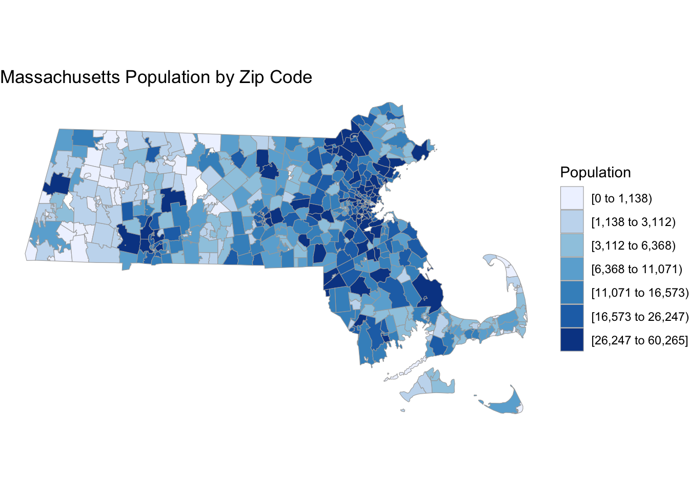
Let’s plot a population choropleth for Massachusetts.
zip_choropleth(
  df_pop_zip,
  state_zoom = "massachusetts",
  title = "Massachusetts Population by Zip Code",
  legend = "Population"
)
 The choropleth object can be further tweaked with ggplot2 functionality.
For more details, check out Ari’s post on Creating ZIP Code Choropleths with choroplethrZip.
Conclusion #
If you have any suggestions, requests, or comments, certainly feel free to drop them below.