Overview #
A circle pack is used to show proportions using circles of different sizes.

The relative positions of the circles don’t mean anything.
Circle packs can be hierarchical, in the sense that categories can be nested within other categories.
Functionally, circle packs are very similar to treemaps. In fact, circle packs are sometimes referred to as “circular treemaps”.
When to use #
Use circle-packs when you want to convey a sense of how different categories compare in terms of scale.
Circle packs aren’t great for precise comparisons, since humans generally aren’t great at visually comparing areas. As an alternative, consider something like a bar plot for precise comparisons.
Circle packs are good for conveying how different categories are nested within other categories (then again, something like this could still be communicated with a stacked bar plot).
Aesthetically, it is a nice change of pace, so if you’re getting bored of treemaps or bar plots, feel free to give circle packs a chance.
Pointers #
Depending on how many circles there are, it’s sometimes visually cleaner to leave details off the smaller circles. Generally, it’s more effective to focus on the big circles and use this sort of plot as a way to focus attention on the most prominent categories being considered.
If there are multiple layers of categories, and the top layer category doesn’t convey too much detail, it might help to just leave the top layer off entirely.
With circle packs, less is often more.
Data #
At a minimum, a circle pack requires a categorical field and a numerical field. When there are only these two fields, then there is no hierarchy to the data, in the sense that there will be no categories nested in other categories.
For instance, a flat, non-hierarchical dataset might look something like this, which is just a made up dataset conveying the number of square feet available on different floors of a house.
| floor | footage |
|---|---|
| first | 900 |
| second | 600 |
| basement | 300 |
The data can also be hierarchical, in the sense that there are sub-categories nested within the major category.
| floor | room | footage |
|---|---|---|
| first | bedroom1 | 450 |
| first | bedroom2 | 300 |
| first | bathroom | 150 |
| second | kitchen | 200 |
| second | dining | 400 |
| basement | utility | 100 |
| basement | storage | 200 |
R #
Circle packs can be generated in R using different packages that build upon ggplot2.
The specific packages that are used depends on whether or not the underlying data is flat or hierarchical.
Flat data #
The simplest package to help generate non-hierchical circle packs in R is the packcircles package.
The packcircles package defines the positions of the circles, and ggplot2 then generates the actual plot.
# install.packages("packcircles") # run if the package isn't already installed
library(packcircles)
Let’s take a look at a flat example dataset.
flat_dat
## # A tibble: 3 × 2
##   floor    footage
##   <chr>      <dbl>
## 1 first        900
## 2 second       600
## 3 basement     300
Now, use the circleProgressiveLayout() function from packcircles to define the positions of the circles.
position <- circleProgressiveLayout(flat_dat$footage, sizetype='area')

position
##             x         y   radius
## 1 -16.9256875   0.00000 16.92569
## 2  13.8197660   0.00000 13.81977
## 3   0.9871775 -19.79643  9.77205
The output defines X coordinates, Y coordinates, and radii for the circles. The radius values are proportional to the original numerical values. In our example, that would be the footage.
These newly-generated values are arranged so that the circles will be positioned so they each barely touch one another without any overlap.
Now it’s time to bind the generated position data with the original flat data.
flat_dat_prep <- cbind(flat_dat, position)

flat_dat_prep
##      floor footage           x         y   radius
## 1    first     900 -16.9256875   0.00000 16.92569
## 2   second     600  13.8197660   0.00000 13.81977
## 3 basement     300   0.9871775 -19.79643  9.77205
Next, we’ll generate another dataset that takes the coordinates and radii and calculates actual point positions of the circles by using the circleLayoutVertices() function.
flat_dat_vertices <- circleLayoutVertices(position, npoints = 50)

head(flat_dat_vertices)
##            x        y id
## 1  0.0000000 0.000000  1
## 2 -0.1334641 2.121351  1
## 3 -0.5317516 4.209247  1
## 4 -1.1885813 6.230761  1
## 5 -2.0935945 8.154012  1
## 6 -3.2325187 9.948670  1
The npoints parameter defines the number of points to be generated per circle. Lines are drawn between the points to form circles. The more points there are, the smoother the circle.
Note that the id field corresponds to unique circles. This field will be used for mappings later when actually generating the plot.
unique(flat_dat_vertices$id)
## [1] 1 2 3
Now it’s time to generate the plot.
ggplot() +
  geom_polygon(
    data = flat_dat_vertices,
    aes(
      x = x,
      y = y,
      group = id,
      fill = as.factor(id) # as.factor makes the id categorical rather than numerical
    )
  )
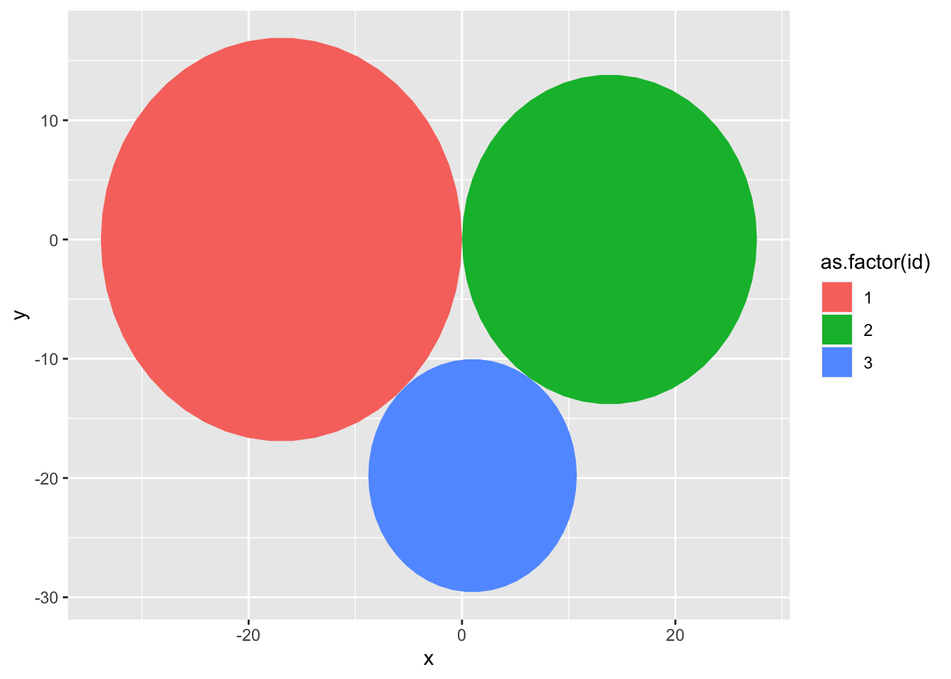
And there we have it: a circle pack. But without labels, it’s kind of useless. While we’re at it, let’s make the label sizes correspond to the square footage.
ggplot() +
  geom_polygon(
    data = flat_dat_vertices,
    aes(
      x = x,
      y = y,
      group = id,
      fill = as.factor(id)
    )
  ) +
  geom_text(
    data = flat_dat_prep,
    aes(
      x = x,
      y = y,
      size = footage,
      label = floor
    )
  )
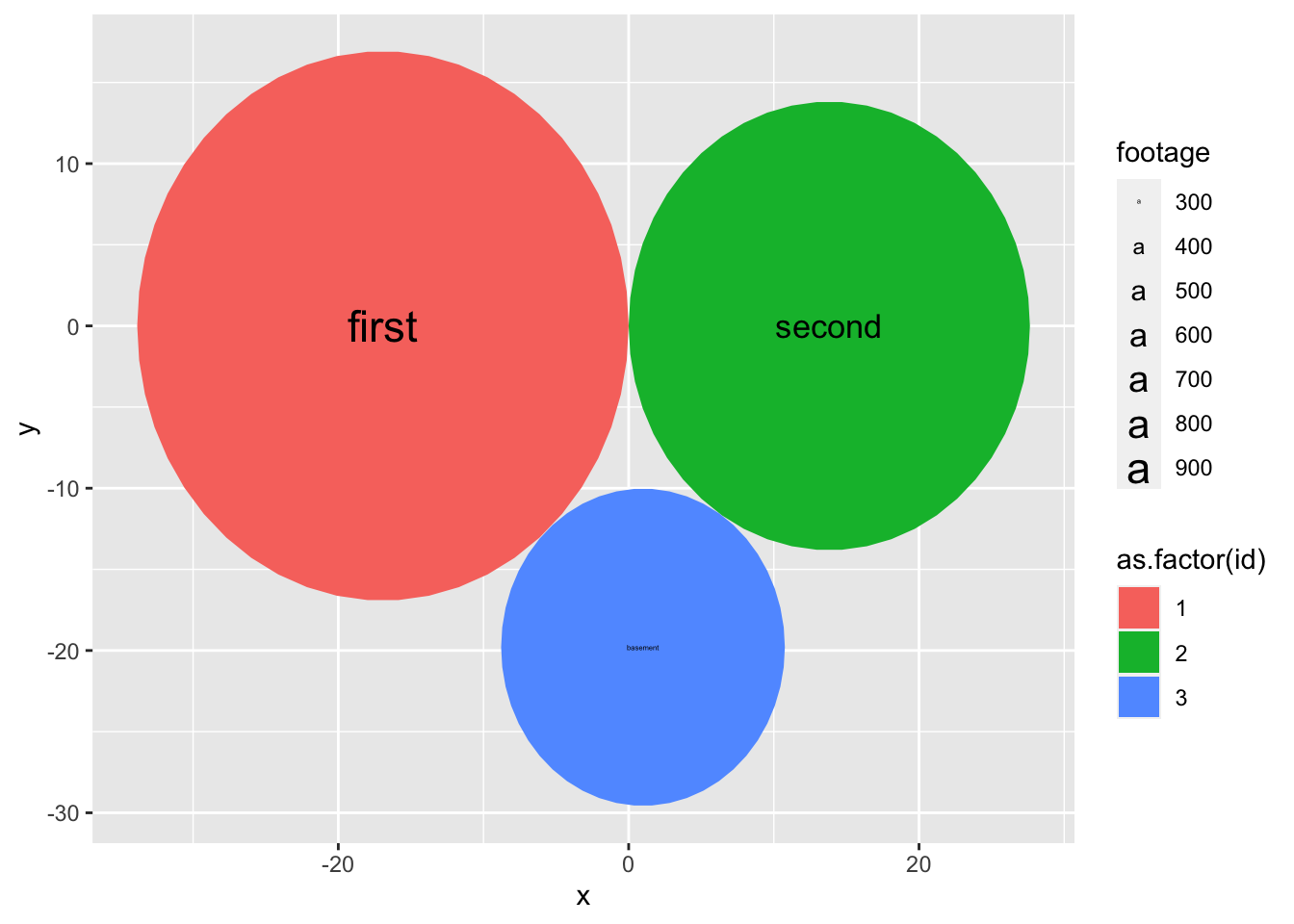
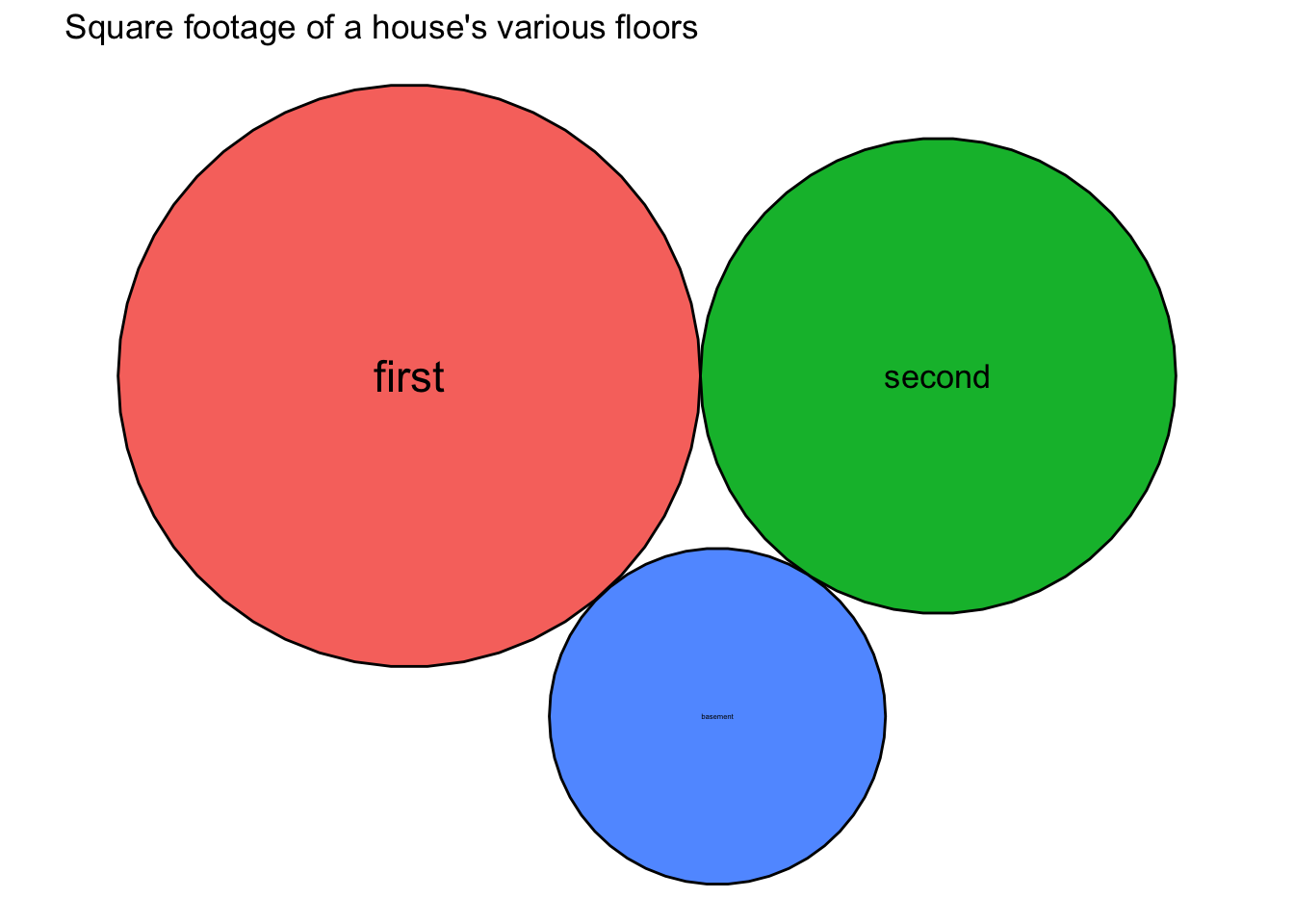
Let’s dress this up with more labels, outlines, dropping extraneous features, and making the coordinate plane equal so the circles look rounder.
ggplot() +
  geom_polygon(
    data = flat_dat_vertices,
    aes(
      x = x,
      y = y,
      group = id,
      fill = as.factor(id)
    ),
    color = "black"
  ) +
  geom_text(
    data = flat_dat_prep,
    aes(
      x = x,
      y = y,
      size = footage,
      label = floor
    )
  ) +
  theme_void() + # switch to a bare theme
  theme(
    legend.position = "none" # get rid of the legend
  ) +
  coord_equal() +
  labs(
    title = "Square footage of a house's various floors"
  )
Hierarchical data #
It’s an entirely different approach when the data is hierarchical.
Hierarchical data can be thought of as graph data. The underlying data should be treated primarily as an edge list, with a “from” column and a “to” column. The “from” column represents the broader category, and the “to” column represents a sub-category.
Let’s look at our previous hierarchical data example.
hierarchical_dat
## # A tibble: 7 × 3
##   floor    room     footage
##   <chr>    <chr>      <dbl>
## 1 first    bedroom1     450
## 2 first    bedroom2     300
## 3 first    bathroom     150
## 4 second   kitchen      200
## 5 second   dining       400
## 6 basement utility      100
## 7 basement storage      200
In this case, the main category is the floor, and the subcategory is the room. Footage is a detail about each room.
We can break this down into an edge list that looks like this:
edges <- select(hierarchical_dat, floor, room) %>%
  rename("from" = "floor", "to" = "room") # rename the column names to edgelist conventions

edges
## # A tibble: 7 × 2
##   from     to
##   <chr>    <chr>
## 1 first    bedroom1
## 2 first    bedroom2
## 3 first    bathroom
## 4 second   kitchen
## 5 second   dining
## 6 basement utility
## 7 basement storage
What this edgelist shows is the floor as the “from”, and the room it contains as the “to”.
We’re only showing one level of nesting, but there could be more. A single “from” category can point to multiple “to” categories.
For instance, “bedroom1” might be a “from”, and its corresponding “to” might be something contained within, like “closet1”.
The vertices (or nodes) are the distinct elements mentioned in the entire edgelist. Oftentimes, vertices will come with additional details.
In our example, the vertices are either the floor or the room, and they each have details about their square footage.
We’ll have to massage the vertices data some to get it into the right form.
rooms <- hierarchical_dat %>%
  select(-floor) %>% # this leaves us with just the room and its square footage
  rename("name" = "room")

floors <- flat_dat %>% # recall that this is just a floor and its corresponding square footage
  rename("name" = "floor")

vertices <- rbind(rooms, floors)

vertices
## # A tibble: 10 × 2
##    name     footage
##    <chr>      <dbl>
##  1 bedroom1     450
##  2 bedroom2     300
##  3 bathroom     150
##  4 kitchen      200
##  5 dining       400
##  6 utility      100
##  7 storage      200
##  8 first        900
##  9 second       600
## 10 basement     300
At this point, we have an edge list and vertices. It’s time to assemble it into a hierchical circular packing plot.
To do so, we’ll use the igraph and ggraph packages, which are useful for handling graph data.
# install.packages(c("igraph", "ggraph")) # run this if the packages haven't already been installed.
library(igraph)
library(ggraph)
First, we have to construct a graph data object by using the graph_from_data_frame() function from igraph.
graph <- graph_from_data_frame(d = edges, vertices = vertices)
Then, we’ll render the circle pack.
ggraph(graph, layout = 'circlepack') +
  geom_node_circle()
## Warning: Using the `size` aesthetic in this geom was deprecated in ggplot2 3.4.0.
## ℹ Please use `linewidth` in the `default_aes` field and elsewhere instead.
## This warning is displayed once every 8 hours.
## Call `lifecycle::last_lifecycle_warnings()` to see where this warning was
## generated.
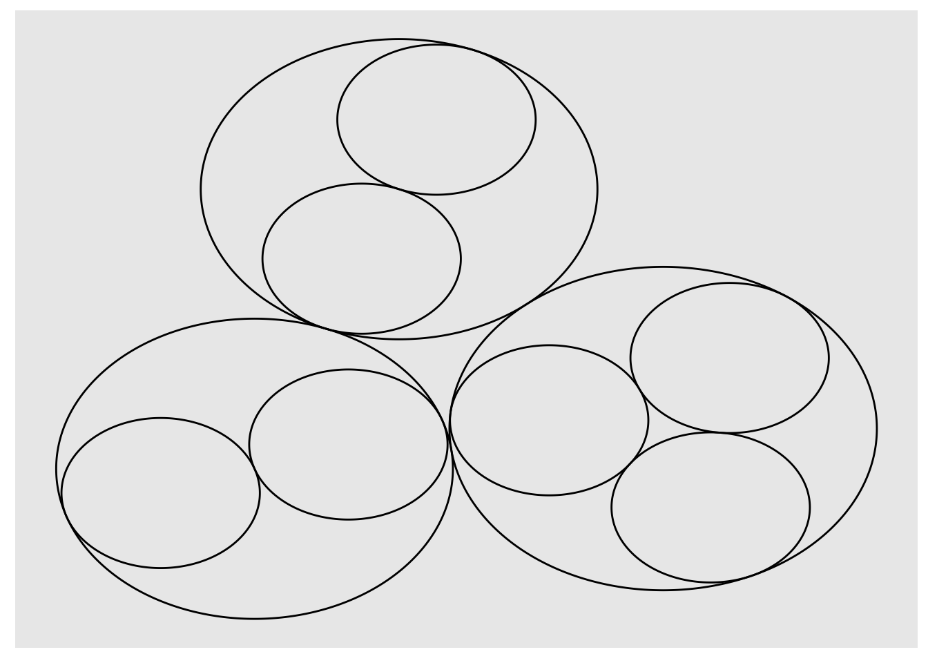
That’s kind of wonky. Let’s slim down the theme, and make the coordinates equal so the shapes are more circular.
ggraph(graph, layout = 'circlepack') +
  geom_node_circle() +
  theme_void() +
  coord_equal()
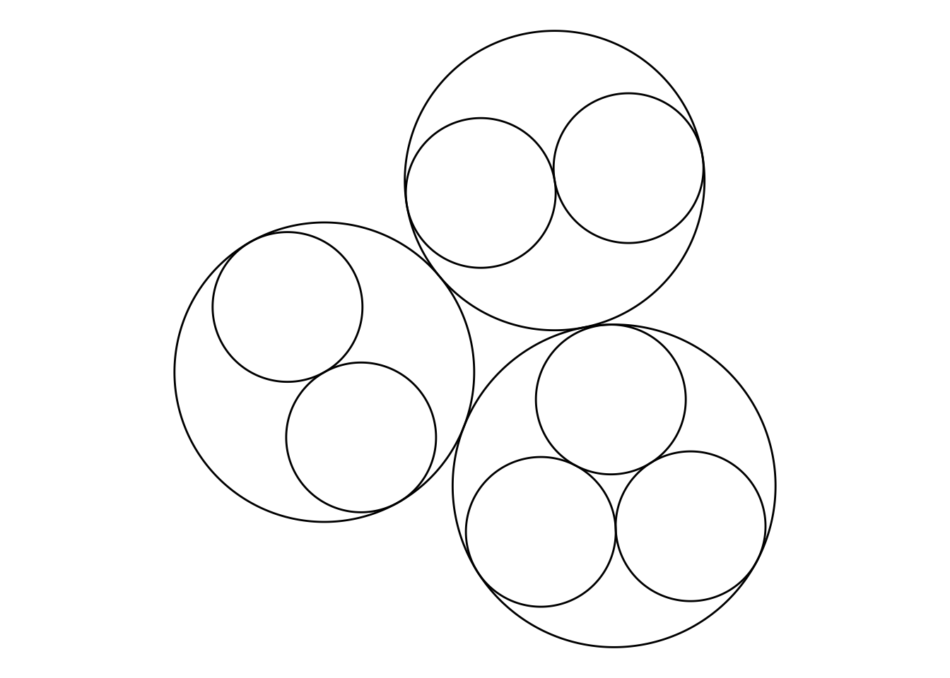
So far, this still isn’t very useful. It needs some labels and maybe some color.
ggraph(graph, layout = 'circlepack') +
  geom_node_circle(aes(fill = depth)) +
  geom_node_text(aes(label = name), color = "white") +
  theme_void() +
  coord_equal()
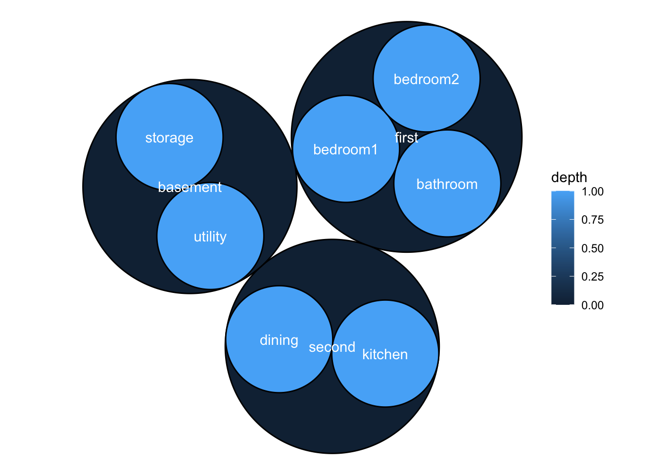
Note that we mapped the fill color to “depth”. Depth refers to how deep down the nesting structure of something is. This is an attribute available to hierarchical data restructured as a graph object.
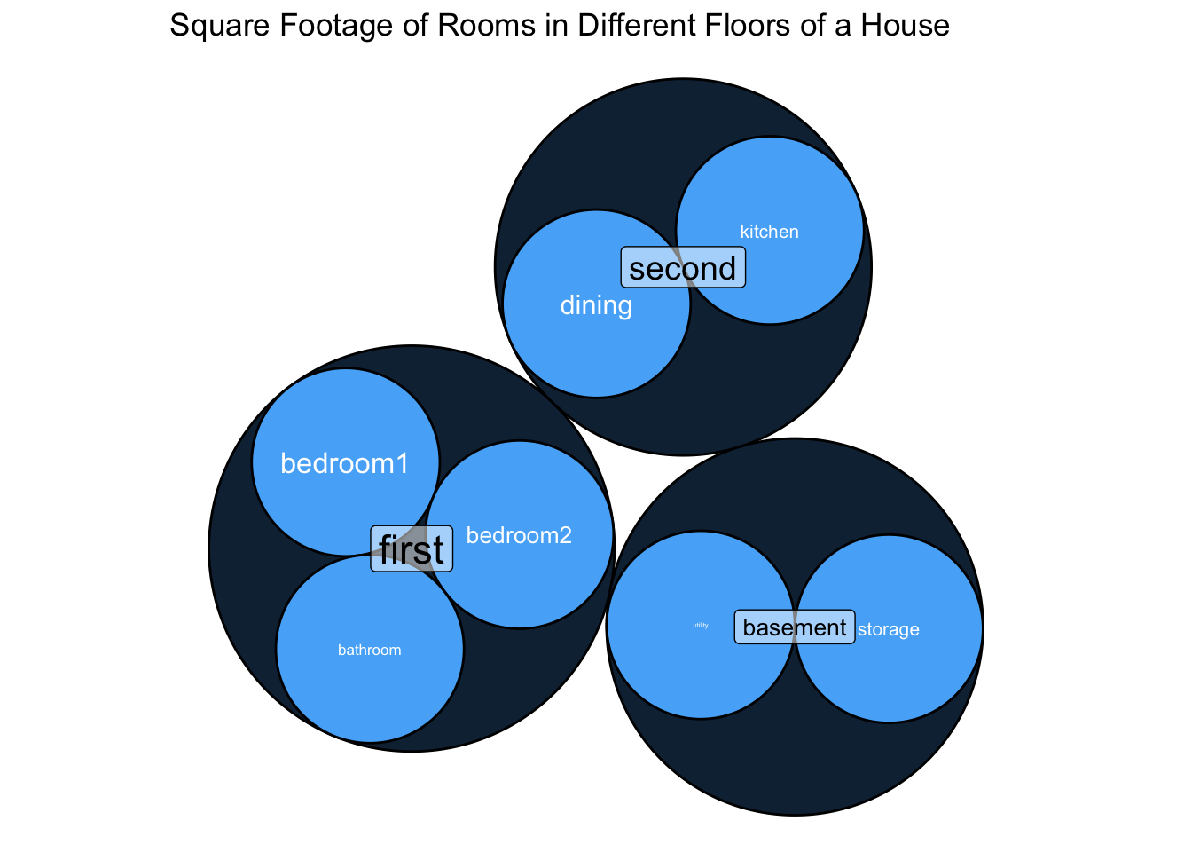
It’s progress, but let’s make this a bit more informative and cleaner. First, let’s add a title. Then, let’s scale the labels to match the corresponding vertex (room or floor).
Let’s also show the lowest level element – the rooms – in white. In graph nomenclature, the lowest level element are leaves (or leaf in singular form).
We’ll keep the label for floors, but make it a dramatically different in design.
ggraph(graph, layout = 'circlepack') +
  geom_node_circle(aes(fill = depth)) +
  geom_node_text(aes(label = name, size = footage, filter = leaf), color = "white") +
  geom_node_label(aes(label = name, size = footage, filter = depth == 0), alpha = .5) +
  theme_void() +
  coord_equal() +
  theme(legend.position = "none") + # remove the legend. We don't need it.
  labs(
    title = "Square Footage of Rooms in Different Floors of a House"
  )
Resources #
Here are some excellent resources on circle packs.