Overview #
A dendrogram is a network diagram that shows the hierarchical relationship between things.
More colloquially, a dendrogram shows how things fit into other things.
Visually, a dendrogram looks like an inverted tree. The language used in referring to parts of a dendrogram follows this tree analogy.
At the very top of the dendrogram is a single node, called the root. The root is considered a commonality across all the observations in the plot.
From this root extends branches. Further down the plot, the branches fork to show that there’s some sort of divergence in characteristics or attributes.
At the very bottom of the dendrogram are the individual observations, called leaves.

The more branches there are between different leaves on a dendogram there are, the less similar the leaves are to one another. Conversely, the fewer branches there are between leaves, the more similar they are.
When to use #
Dendrograms are commonly used to show hierarchical data or the results of hierarchical clustering.
Hierarchical data is structured in a way to show how some things fit into or roll up into other things. I believe this is fairly straightforward. Think of organizational structures as a prime example.
Hierarchical clustering is a data science method that tries to find groupings within raw data without relying on any specific training data. It works by trying to find commonalities across individual data points based on their attributes, and draws connections between those data points based on commonalities.
On a dendrogram, data points with few branches between them might be grouped together as a common cluster.
I’ll save a more in-depth coverage of hierarchical clustering for another post.
Data #
The data that we can use to construct a dendogram needs to be nested in some way.
One format is an edgelist, which includes fields usually named “from” and “to”. This is the same sort of data structure that we would use with a circle pack.
One way to think of this is that each “from” points to a “to” that is contained within the “from”. The “to” in one record on the edgelist might be the “from” on another record on the edgelist.
Let’s use a house dataset as an example. The house might have multiple floors, and each floor might have multiple rooms.
| from | to |
|---|---|
| house | first floor |
| house | second floor |
| house | basement |
| first floor | kitchen |
| first floor | living room |
| first floor | foyer |
| first floor | half bath |
| second floor | master bedroom |
| second floor | second room |
| second floor | guest room |
| basement | utilities |
| basement | storage |
R #
The easiest way to construct a dendrogram in R is to use ggraph by Thomas Lin Pedersen, which builds upon igraph and ggplot2.
library(ggraph)
library(igraph)

library(tidyverse) # which also includes ggplot2
Let’s re-create the data example from above.
example <- tribble(
  ~from, ~to,
  "house", "first floor",
  "house", "second floor",
  "house", "basement",
  "first floor", "kitchen",
  "first floor", "living room",
  "first floor", "foyer",
  "first floor", "half bath",
  "second floor", "master bedroom",
  "second floor", "second room",
  "second floor", "guest room",
  "basement", "utilities",
  "basement", "storage"
)

example
## # A tibble: 12 × 2
##    from         to
##    <chr>        <chr>
##  1 house        first floor
##  2 house        second floor
##  3 house        basement
##  4 first floor  kitchen
##  5 first floor  living room
##  6 first floor  foyer
##  7 first floor  half bath
##  8 second floor master bedroom
##  9 second floor second room
## 10 second floor guest room
## 11 basement     utilities
## 12 basement     storage
Now convert that example data into a graph object to be used in what is fundamentally a network graph plot.
graph <- igraph::graph_from_data_frame(example)
Let’s turn that into a dendrogram.
ggraph(graph, layout = 'dendrogram') +
  geom_edge_diagonal() +
  geom_node_point()
## Warning: Using the `size` aesthetic in this geom was deprecated in ggplot2 3.4.0.
## ℹ Please use `linewidth` in the `default_aes` field and elsewhere instead.
## This warning is displayed once every 8 hours.
## Call `lifecycle::last_lifecycle_warnings()` to see where this warning was
## generated.
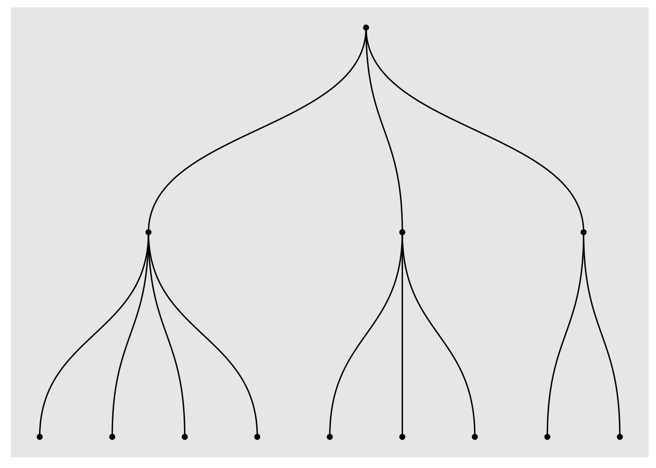
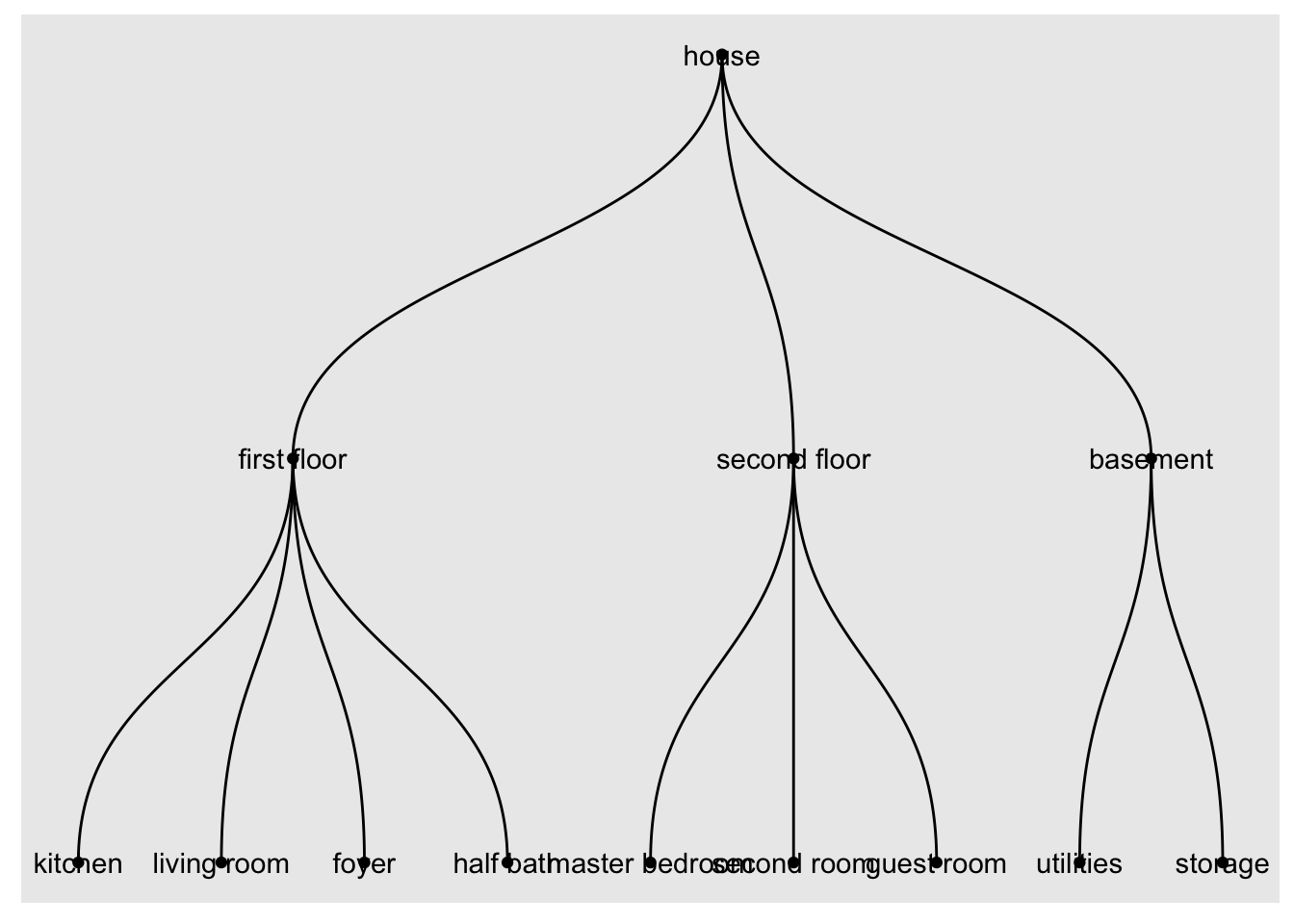
Without labels, that’s pretty useless. We can add labels with the geom_node_text() function, and map the label aesthetic to name. The name element is an attribute that’s embedded within the graph data when we called the graph_from_data_frame() function earlier.
ggraph(graph, layout = 'dendrogram') +
  geom_edge_diagonal() +
  geom_node_point() +
  geom_node_text(aes(label = name))
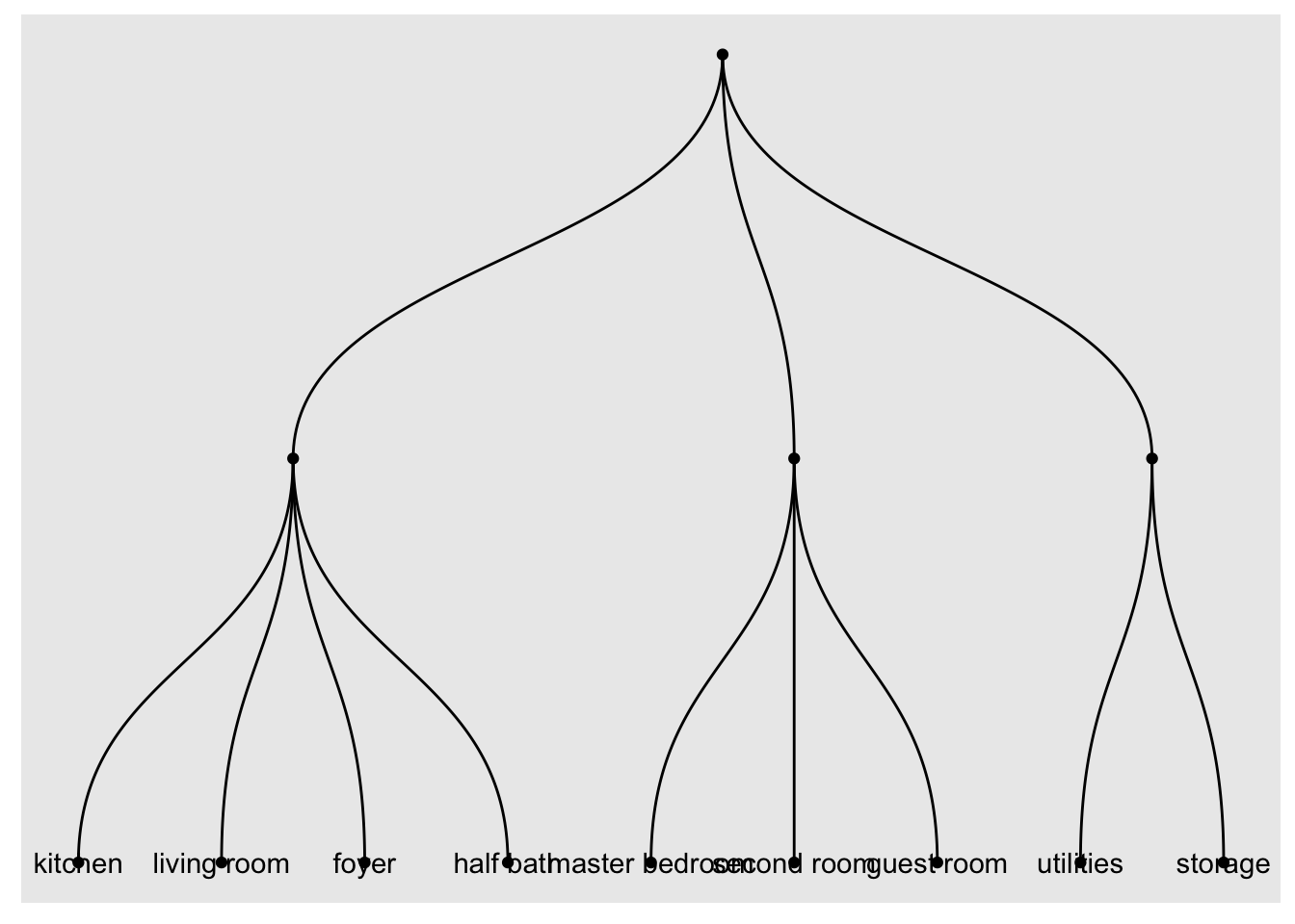
For demonstration purposes, we can filter this down to only the leaves. But we’re not going to keep that because I do think it’s useful to show other nodes as well.
ggraph(graph, layout = 'dendrogram') +
  geom_edge_diagonal() +
  geom_node_point() +
  geom_node_text(aes(label = name, filter=leaf))
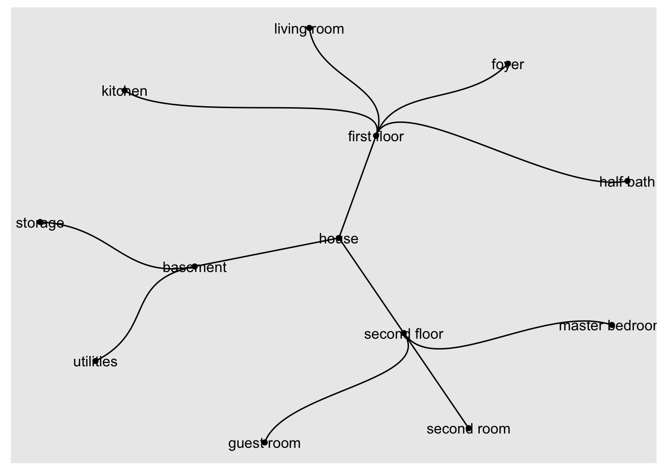
We can also turn this into a circular dendrogram.
ggraph(graph, layout = 'dendrogram', circular = TRUE) +
  geom_edge_diagonal() +
  geom_node_point() +
  geom_node_text(aes(label = name))
For now, let’s go back to the original dendrogram with labels, and polish it up some. Instead of text on points, let’s switch it to geom_node_label, which is labels in containers. This I think provides a cleaner look in this case. Let’s also add a few other enhancements.
ggraph(graph, layout = 'dendrogram') +
  geom_edge_diagonal() +
  geom_node_point() +
  geom_node_label(aes(label = name)) +
  theme_void() + # a very bare theme
  labs(
    title = "A Dendrogram of a House"
  )
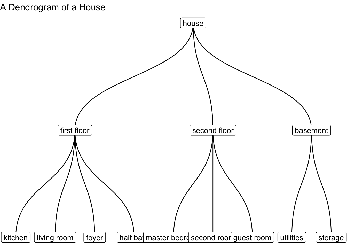
That’s it – a bare bones dendrogram from hierarchical data.